PyRTL
PyRTL is a Python library for register-transfer-level hardware design and simulation. Get started with:
$ pip install pyrtl
Features
PyRTL provides a collection of classes for Pythonic register-transfer level design, simulation, tracing, and testing suitable for teaching and research. Simplicity, usability, clarity, and extensibility are overarching goals, rather than performance or optimization. Features include:
Elaboration-through-execution, meaning all of Python can be used, including introspection.
Design, instantiate, and simulate all in one file, and without leaving Python.
Export to, or import from, common HDLs (BLIF-in, Verilog-out currently supported).
Examine execution with waveforms in a terminal or export to .vcd as projects scale.
Elaboration, synthesis, and basic optimizations all included.
Small and well-defined internal core structure means writing new transforms is easier.
Batteries included means many useful components are already available.
The new pyrtl.rtllib.float module generates floating point hardware!
Simple Examples
Here are some simple examples of PyRTL in action. These examples implement the same functionality as those highlighted in the wonderful related work Chisel, which in turn allows us to see the stylistic differences between the approaches.
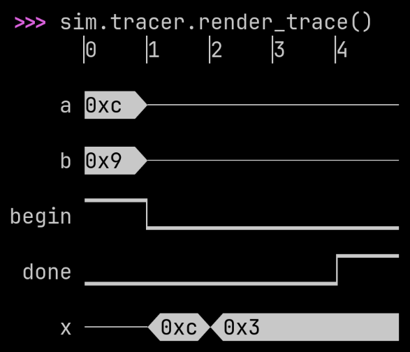
A greatest common denominator calculator: gcd generates a sequential
circuit that saves inputs a and b when begin goes high, and
then, while begin is low, calculates the GCD with Euclid’s algorithm. The function
returns two WireVectors, one which holds the
GCD when the computation is done, and the other which is a boolean
done signal.
The code below provides everything needed to instantiate, simulate, and visualize the resulting design.
import pyrtl

# # Greatest common denominator example.


def gcd(
    a: pyrtl.WireVector, b: pyrtl.WireVector, begin: pyrtl.WireVector
) -> tuple[pyrtl.WireVector, pyrtl.WireVector]:
    x = pyrtl.Register(bitwidth=a.bitwidth)
    y = pyrtl.Register(bitwidth=b.bitwidth)
    done = pyrtl.WireVector(bitwidth=1)

    with pyrtl.conditional_assignment:
        with begin:
            x.next |= a
            y.next |= b
        with x > y:
            x.next |= x - y
        with y > x:
            y.next |= y - x
        with pyrtl.otherwise:
            done |= True
    return x, done


a = pyrtl.Input(name="a", bitwidth=8)
b = pyrtl.Input(name="b", bitwidth=8)
begin = pyrtl.Input(name="begin", bitwidth=1)

x = pyrtl.Output(name="x", bitwidth=8)
done = pyrtl.Output(name="done", bitwidth=1)

x_, done_ = gcd(a, b, begin)
x <<= x_
done <<= done_

# Simulate the design.
sim = pyrtl.Simulation()
sim.step({"a": 12, "b": 9, "begin": True})
while not sim.inspect("done"):
    sim.step({"a": 0, "b": 0, "begin": False})
sim.tracer.render_trace()
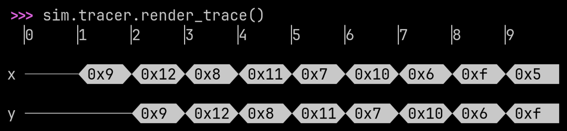
A finite impulse response filter: fir generates a sequential circuit
that accepts inputs x and a list of coefficients bs. From the
Wikipedia FIR description, the list
zs is the registers required to implement the delay. fir returns
an output y which is the resulting sum of products and is valid every
cycle (since the design is naturally fully pipelined).
import pyrtl

# # Finite impulse response filter example.


def fir(x: pyrtl.WireVector, bs: list[int]):
    rwidth = x.bitwidth  # Bitwidth of the registers.
    ntaps = len(bs)  # Number of coefficients.

    zs = [x] + [pyrtl.Register(rwidth) for _ in range(ntaps - 1)]
    for i in range(1, ntaps):
        zs[i].next <<= zs[i - 1]

    # Produce the final sum of products.
    return sum(z * b for z, b in zip(zs, bs, strict=True))


x = pyrtl.Input(name="x", bitwidth=8)
y = pyrtl.Output(name="y", bitwidth=8)
y <<= fir(x, bs=[0, 1])

# Simulate the design.
sim = pyrtl.Simulation()
sim.step_multiple({"x": [0, 9, 18, 8, 17, 7, 16, 6, 15, 5]})
sim.tracer.render_trace()
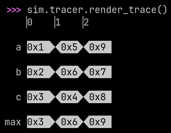
max_n generates hardware that identifies the largest of N input
values. This example makes use of Python’s notation for handling
multiple inputs
by packing them into a list. It also demonstrates that the full
power of Python is available to you in PyRTL, including functional tools
like reduce(), which is used to chain together multiple
max_2 elements into a bigger max_n.
from functools import reduce

import pyrtl

# # N-way max example.


def max_n(*inputs):
    def max_2(x, y):
        return pyrtl.select(x > y, x, y)

    return reduce(max_2, inputs)


a = pyrtl.Input(name="a", bitwidth=8)
b = pyrtl.Input(name="b", bitwidth=8)
c = pyrtl.Input(name="c", bitwidth=8)
max = pyrtl.Output(name="max", bitwidth=8)

max <<= max_n(a, b, c)

# Simulate the design.
sim = pyrtl.Simulation()
sim.step_multiple({"a": [1, 5, 9], "b": [2, 6, 7], "c": [3, 4, 8]})
sim.tracer.render_trace()
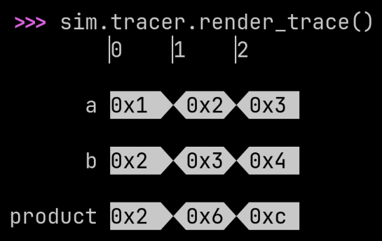
mul generates a small 4 x 4 multiplier with a simple ROM lookup. The first two
lines simply check that the inputs are each 4-bits wide. romdata is a
Python function that calculates the values we want stored in the ROM, as
a function of the ROM address. RomBlock automatically
initializes the ROM with values computed by romdata. The generated
hardware simply concats the two 4-bit inputs into
an 8-bit ROM address and returns the value stored in the ROM at that
address.
import pyrtl

# # ROM-based multiplier example.


def mul(x: pyrtl.WireVector, y: pyrtl.WireVector) -> pyrtl.WireVector:
    assert x.bitwidth == 4
    assert y.bitwidth == 4

    def romdata(addr: int) -> int:
        return (addr >> 4) * (addr & 0xF)

    tbl = pyrtl.RomBlock(bitwidth=8, addrwidth=8, romdata=romdata)
    return tbl[pyrtl.concat(x, y)]


a = pyrtl.Input(name="a", bitwidth=4)
b = pyrtl.Input(name="b", bitwidth=4)
product = pyrtl.Output(name="product", bitwidth=8)

product <<= mul(a, b)

# Simulate the design.
sim = pyrtl.Simulation()
sim.step_multiple({"a": [1, 2, 3], "b": [2, 3, 4]})
sim.tracer.render_trace()
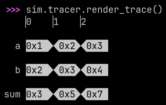
The classic ripple-carry adder: adder generates a ripple carry adder
of arbitrary length including both carry in and carry out. The full
adder
(fa) takes 1-bit inputs and produces 1-bit outputs. We iteratively
create full adders and link the carry in of each new full adder to the
carry out of the last full adder. adder’s sum is a Python
list that keeps track of the wires carrying the sum bits. The
final full_sum is produced by concatenating the wires in sum with
concat_list().
import pyrtl

# # Ripple-carry adder example.


def fa(
    x: pyrtl.WireVector, y: pyrtl.WireVector, cin: pyrtl.WireVector
) -> tuple[pyrtl.WireVector, pyrtl.WireVector]:
    """Full adder."""
    sum = x ^ y ^ cin
    cout = x & y | y & cin | x & cin
    return sum, cout


def adder(
    a: pyrtl.WireVector, b: pyrtl.WireVector, cin: pyrtl.WireVector
) -> tuple[pyrtl.WireVector, pyrtl.WireVector]:
    """n-bit ripple carry adder with carry in and carry out."""
    a, b = pyrtl.match_bitwidth(a, b)

    sum = [None] * a.bitwidth
    for i in range(a.bitwidth):
        sum[i], cout = fa(a[i], b[i], cin)
        cin = cout

    full_sum = pyrtl.concat_list(sum)
    return full_sum, cout


a = pyrtl.Input(name="a", bitwidth=4)
b = pyrtl.Input(name="b", bitwidth=4)
sum = pyrtl.Output(name="sum", bitwidth=8)

sum_, cout_ = adder(a, b, pyrtl.Const(0))
sum <<= sum_

# Simulate the design.
sim = pyrtl.Simulation()
sim.step_multiple({"a": [1, 2, 3], "b": [2, 3, 4]})
sim.tracer.render_trace()
The 10,000 Foot Overview
At a high level, PyRTL builds hardware that you explicitly define. If you are looking for a tool to take your random Python code and turn it into hardware, you will have to look elsewhere: this is not HLS. Instead, PyRTL helps you concisely and precisely describe a digital hardware structure, which you already have worked out in detail, in Python.
PyRTL restricts you to a set of reasonable digital designs practices: the clock and resets are implicit, block memories are synchronous by default, there are no “undriven” states, and un-registered feedback loops are not allowed. Instead of worrying about these “analog-ish” tricks that are horrible ideas in modern processes anyways, PyRTL lets you treat hardware design like a software problem: build recursive hardware, write introspective containers, and have fun building digital designs again!
To the user it provides a set of Python classes that allow them to Pythonically
express their hardware designs. For example, with WireVector
you get a structure that acts very much like a Python list of 1-bit wires, so
mywire[:-1] selects everything except the most-significant-bit. Of course
you can add, subtract, and multiply
these WireVectors, or concat() multiple
bit-vectors end-to-end as well.
You can even put WireVectors in Python collections
and process them in bulk. For example, if x is a list of
WireVectors, and you want to multiply each of them
by 2 and sum them into a WireVector y:
y = sum([elem * 2 for elem in x])
Hardware comprehensions are surprisingly useful. We’ll cover an example in more detail below, but if you just want to play around with PyRTL, try our examples in your browser.
Hello N-bit Ripple-Carry Adder!
While adders are a builtin primitive for PyRTL, most people writing RTL are familiar with Ripple-Carry Adders and so it is useful to see how you might express one in PyRTL. Rather than the typical Verilog introduction to fixed 4-bit adders, let’s go ahead and build an arbitrary bitwidth adder.
import pyrtl

# # Ripple-carry adder example.


def one_bit_add(
    a: pyrtl.WireVector, b: pyrtl.WireVector, carry_in: pyrtl.WireVector | int
) -> tuple[pyrtl.WireVector, pyrtl.WireVector]:
    assert len(a) == len(b) == 1  # `len` returns the bitwidth.
    sum = a ^ b ^ carry_in  # WireVector operators build the hardware.
    carry_out = a & b | a & carry_in | b & carry_in
    return sum, carry_out


def ripple_add(
    a: pyrtl.WireVector, b: pyrtl.WireVector, carry_in: pyrtl.WireVector | int = 0
) -> tuple[pyrtl.WireVector, pyrtl.WireVector]:
    a, b = pyrtl.match_bitwidth(a, b)
    if len(a) == 1:
        sumbits, carry_out = one_bit_add(a, b, carry_in)
    else:
        lsbit, ripplecarry = one_bit_add(a[0], b[0], carry_in)
        msbits, carry_out = ripple_add(a[1:], b[1:], ripplecarry)
        sumbits = pyrtl.concat(msbits, lsbit)
    return sumbits, carry_out


# Use the adder in a 3-bit counter.
counter = pyrtl.Register(bitwidth=3, name="counter")
sum, _carry_out = ripple_add(counter, pyrtl.Const(1))
counter.next <<= sum

# Simulate the instantiated design for 12 cycles.
sim = pyrtl.Simulation()
sim.step_multiple(nsteps=12)
sim.tracer.render_trace()
The code above includes ripple_add, an adder generator with Python-style
slices on wires, counter, an instance of Register, and all
the code needed to simulate the design, generate a waveform, and render it to
the terminal. Example 2
has more comments on how this code works. Running this code shows a counter
running from 0 to 7 and repeating:
